Exploring Supervised Machine Learning Algorithms

The main goal of this reading is to understand enough statistical methodology to be able to leverage the machine learning algorithms in Python’s scikit-learn library and then apply this knowledge to solve a classic machine learning problem.

The first stop of our journey will take us through a brief history of machine learning. Then we will dive into different algorithms. On our final stop, we will use what we learned to solve the Titanic Survival Rate Prediction Problem.

Some disclaimers:

• I am a full-stack software engineer, not a machine learning algorithm expert.
• I assume you know some basic Python.
• This is exploratory, so not every detail is explained like it would be in a tutorial.

With that noted, let’s dive in!

A Quick Introduction to Machine Learning Algorithms

As soon as you venture into this field, you realize that machine learning is less romantic than you may think. Initially, I was full of hopes that after I learned more I would be able to construct my own Jarvis AI, which would spend all day coding software and making money for me, so I could spend whole days outdoors reading books, driving a motorcycle, and enjoying a reckless lifestyle while my personal Jarvis makes my pockets deeper. However, I soon realized that the foundation of machine learning algorithms is statistics, which I personally find dull and uninteresting. Fortunately, it did turn out that “dull” statistics have some very fascinating applications.

You will soon discover that to get to those fascinating applications, you need to understand statistics very well. One of the goals of machine learning algorithms is to find statistical dependencies in supplied data.

The supplied data could be anything from checking blood pressure against age to finding handwritten text based on the color of various pixels.

That said, I was curious to see if I could use machine learning algorithms to find dependencies in cryptographic hash functions (SHA, MD5, etc.)—however, you can’t really do that because proper crypto primitives are constructed in such a way that they eliminate dependencies and produce significantly hard-to-predict output. I believe that, given an infinite amount of time, machine learning algorithms could crack any crypto model.

Unfortunately, we don’t have that much time, so we need to find another way to efficiently mine cryptocurrency. How far have we gotten up until now?

A Brief History of Machine Learning Algorithms

The roots of machine learning algorithms come from Thomas Bayes, who was English statistician who lived in the 18th century. His paper An Essay Towards Solving a Problem in the Doctrine of Chances underpins Bayes’ Theorem, which is widely applied in the field of statistics.

In the 19th century, Pierre-Simon Laplace published Théorie analytique des probabilités, expanding on the work of Bayes and defining what we know of today as Bayes’ Theorem. Shortly before that, Adrien-Marie Legendre had described the “least squares” method, also widely used today in supervised learning.

The 20th century is the period when the majority of publicly known discoveries have been made in this field. Andrey Markov invented Markov chains, which he used to analyze poems. Alan Turing proposed a learning machine that could become artificially intelligent, basically foreshadowing genetic algorithms. Frank Rosenblatt invented the Perceptron, sparking huge excitement and great coverage in the media.

But then the 1970s saw a lot of pessimism around the idea of AI—and thus, reduced funding—so this period is called an AI winter. The rediscovery of backpropagation in the 1980s caused a resurgence in machine learning research. And today, it’s a hot topic once again.

The late Leo Breiman distinguished between two statistical modeling paradigms: Data modeling and algorithmic modeling. “Algorithmic modeling” means more or less the machine learning algorithms like the random forest.

Machine learning and statistics are closely related fields. According to Michael I. Jordan, the ideas of machine learning, from methodological principles to theoretical tools, have had a long prehistory in statistics. He also suggested data science as a placeholder term for the overall problem that machine learning specialists and statisticians are both implicitly working on.

Categories of Machine Learning Algorithms

The machine learning field stands on two main pillars called supervised learning and unsupervised learning. Some people also consider a new field of study—deep learning—to be separate from the question of supervised vs. unsupervised learning.

Supervised learning is when a computer is presented with examples of inputs and their desired outputs. The goal of the computer is to learn a general formula which maps inputs to outputs. This can be further broken down into:

• Semi-supervised learning, which is when the computer is given an incomplete training set with some outputs missing
• Active learning, which is when the computer can only obtain training labels for a very limited set of instances. When used interactively, their training sets can be presented to the user for labeling.
• Reinforcement learning, which is when the training data is only given as feedback to the program’s actions in the dynamic environment, such as driving a vehicle or playing a game against an opponent

In contrast, unsupervised learning is when no labels are given at all and it’s up to the algorithm to find the structure in its input. Unsupervised learning can be a goal in itself when we only need to discover hidden patterns.

Deep learning is a new field of study which is inspired by the structure and function of the human brain and based on artificial neural networks rather than just statistical concepts. Deep learning can be used in both supervised and unsupervised approaches.

In this article, we will only go through some of the simpler supervised machine learning algorithms and use them to calculate the survival chances of an individual in tragic sinking of the Titanic. But in general, if you’re not sure which algorithm to use, a nice place to start is scikit-learn’s machine learning algorithm cheat-sheet.

Basic Supervised Machine Learning Models

Perhaps the easiest possible algorithm is linear regression. Sometimes this can be graphically represented as a straight line, but despite its name, if there’s a polynomial hypothesis, this line could instead be a curve. Either way, it models the relationships between scalar dependent variable $y$ and one or more explanatory values denoted by $x$.

In layperson’s terms, this means that linear regression is the algorithm which learns the dependency between each known $x$ and $y$, such that later we can use it to predict $y$ for an unknown sample of $x$.

In our first supervised learning example, we will use a basic linear regression model to predict a person’s blood pressure given their age. This is a very simple dataset with two meaningful features: Age and blood pressure.

As already mentioned above, most machine learning algorithms work by finding a statistical dependency in the data provided to them. This dependency is called a hypothesis and is usually denoted by $h\left(\theta \right)$.

To figure out the hypothesis, let’s start by loading and exploring the data.

import matplotlib.pyplot as plt
from pandas import read_csv
import os

# Load data
data_path = os.path.join(os.getcwd(), "data/blood-pressure.txt")
dataset = read_csv(data_path, delim_whitespace=True)

# We have 30 entries in our dataset and four features. The first feature is the ID of the entry.
# The second feature is always 1. The third feature is the age and the last feature is the blood pressure.
# We will now drop the ID and One feature for now, as this is not important.
dataset = dataset.drop(['ID', 'One'], axis=1)

# And we will display this graph
%matplotlib inline
dataset.plot.scatter(x='Age', y='Pressure')

# Now, we will assume that we already know the hypothesis and it looks like a straight line
h = lambda x: 84 + 1.24 * x

# Let's add this line on the chart now
ages = range(18, 85)
estimated = []

for i in ages:
    estimated.append(h(i))

plt.plot(ages, estimated, 'b')  

[]

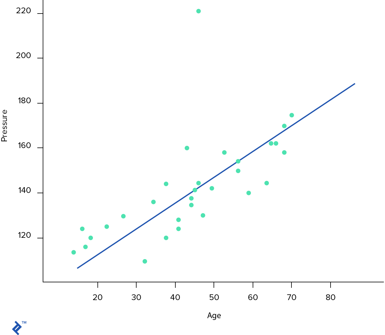
On the chart above, every blue dot represents our data sample and the blue line is the hypothesis which our algorithm needs to learn. So what exactly is this hypothesis anyway?

In order to solve this problem, we need to learn the dependency between $x$ and $y$, which is denoted by $y=f\left(x\right)$. Therefore $f\left(x\right)$ is the ideal target function. The machine learning algorithm will try to guess the hypothesis function $h\left(x\right)$ that is the closest approximation of the unknown $f\left(x\right)$.

The simplest possible form of hypothesis for the linear regression problem looks like this: $h_{\theta }\left(x\right)={\theta }_0+{\theta }_1\ast x$. We have a single input scalar variable $x$ which outputs a single scalar variable $y$, where ${\theta }_0$ and ${\theta }_1$ are parameters which we need to learn. The process of fitting this blue line in the data is called linear regression. It is important to understand that we have only one input parameter $x_1$; however, a lot of hypothesis functions will also include the bias unit ($x_0$). So our resulting hypothesis has a form of $h_{\theta }\left(x\right)={\theta }_0\ast x_0+{\theta }_1\ast x_1$. But we can avoid writing $x_0$ because it’s almost always equal to 1.

Getting back to the blue line. Our hypothesis looks like $h\left(x\right)=84+1.24x$, which means that ${\theta }_0=84$ and ${\theta }_1=1.24$. How can we automatically derive those $\theta$ values?

We need to define a cost function. Essentially, what cost function does is simply calculates the root mean square error between the model prediction and the actual output.

$$J\left(\theta \right)=\frac{1}{2m}\sum _{i=1}^m\left(h_{\theta }\right(x^{\left(i\right)})-y^{\left(i\right)}{)}^2$$

For example, our hypothesis predicts that for someone who is 48 years old, their blood pressure should be $h\left(48\right)=84+1.24\ast 48=143mmHg$; however, in our training sample, we have the value of $130mmHg$. Therefore the error is $(143-130{)}^2=169$. Now we need to calculate this error for every single entry in our training dataset, then sum it together (${\sum }_{i=1}^m\left(h_{\theta }\right(x^{\left(i\right)})-y^{\left(i\right)}{)}^2$) and take the mean value out of that.

This gives us a single scalar number which represents the cost of the function. Our goal is to find $\theta$ values such that the cost function is the lowest; in the other words, we want to minimize the cost function. This will hopefully seem intuitive: If we have a small cost function value, this means that the error of prediction is small as well.

import numpy as np
# Let's calculate the cost for the hypothesis above

h = lambda x, theta_0, theta_1: theta_0 + theta_1 * x

def cost(X, y, t0, t1):
    m = len(X) # the number of the training samples
    c = np.power(np.subtract(h(X, t0, t1), y), 2)
    return (1 / (2 * m)) * sum(c)

X = dataset.values[:, 0]
y = dataset.values[:, 1]
print('J(Theta) = %2.2f' % cost(X, y, 84, 1.24))

J(Theta) = 1901.95

Now, we need to find such values of $\theta$ such that our cost function value is minimal. But how do we do that?

$$minJ\left(\theta \right)=\frac{1}{2m}\sum _{i=1}^m\left(h_{\theta }\right(x^{\left(i\right)})-y^{\left(i\right)}{)}^2$$

There are several possible algorithms, but the most popular is gradient descent. In order to understand the intuition behind the gradient descent method, let’s first plot it on the graph. For the sake of simplicity, we will assume a simpler hypothesis $h\left(\theta \right)={\theta }_1\ast x$. Next, we will plot a simple 2D chart where $x$ is the value of $\theta$ and $y$ is the cost function at this point.

import matplotlib.pyplot as plt

fig = plt.figure()

# Generate the data
theta_1 = np.arange(-10, 14, 0.1)

J_cost = []
for t1 in theta_1:
    J_cost += [ cost(X, y, 0, t1) ]

plt.plot(theta_1, J_cost)

plt.xlabel(r'$\theta_1$')
plt.ylabel(r'$J(\theta)$')

plt.show()

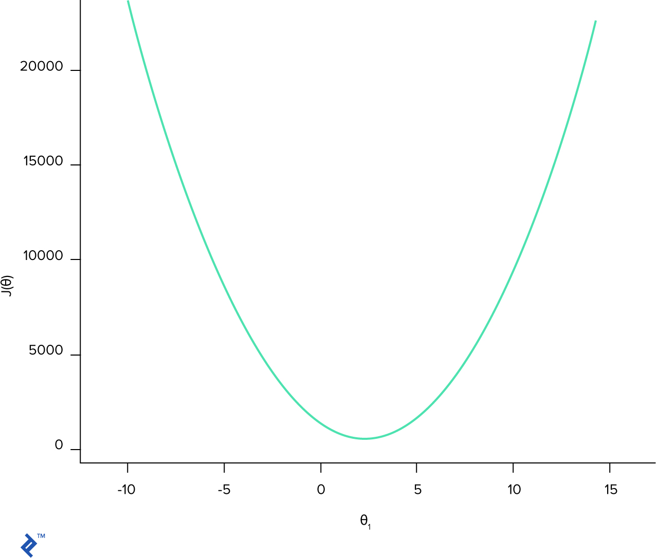
The cost function is convex, which means that on the interval $[a,b]$ there is only one minimum. Which again means that the best $\theta$ parameters are at the point where the cost function is minimal.

Basically, gradient descent is an algorithm that tries to find the set of parameters which minimize the function. It starts with an initial set of parameters and iteratively takes steps in the negative direction of the function gradient.

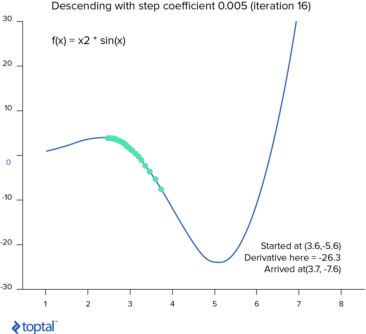
If we calculate the derivative of a hypothesis function at a specific point, this will give us a slope of the tangent line to the curve at that point. This means that we can calculate the slope at every single point on the graph.

The way the algorithm works is this:

1. We choose a random starting point (random $\theta$).
2. Calculate the derivative of the cost function at this point.
3. Take the small step towards the slope ${\theta }_j:={\theta }_j-\lambda \ast \frac{\partial }{\partial {\theta }_j}\ast J\left(\theta \right)$.
4. Repeat steps 2-3 until we converge.

Now, the convergence condition depends on the implementation of the algorithm. We may stop after 50 steps, after some threshold, or anything else.

import math
# Example of the simple gradient descent algorithm taken from Wikipedia

cur_x = 2.5 # The algorithm starts at point x
gamma = 0.005 # Step size multiplier
precision = 0.00001
previous_step_size = cur_x

df = lambda x: 2 * x * math.cos(x)

# Remember the learning curve and plot it 

while previous_step_size > precision:
    prev_x = cur_x
    cur_x += -gamma * df(prev_x)
    previous_step_size = abs(cur_x - prev_x)

print("The local minimum occurs at %f" % cur_x)

The local minimum occurs at 4.712194

We will not implement those algorithms in this article. Instead, we will utilize the widely adopted scikit-learn, an open-source Python machine learning library. It provides a lot of very useful APIs for different data mining and machine learning problems.

from sklearn.linear_model import LinearRegression
# LinearRegression uses the gradient descent method

# Our data
X = dataset[['Age']]
y = dataset[['Pressure']]

regr = LinearRegression()
regr.fit(X, y)

# Plot outputs
plt.xlabel('Age')
plt.ylabel('Blood pressure')

plt.scatter(X, y,  color='black')
plt.plot(X, regr.predict(X), color='blue')

plt.show()
plt.gcf().clear()

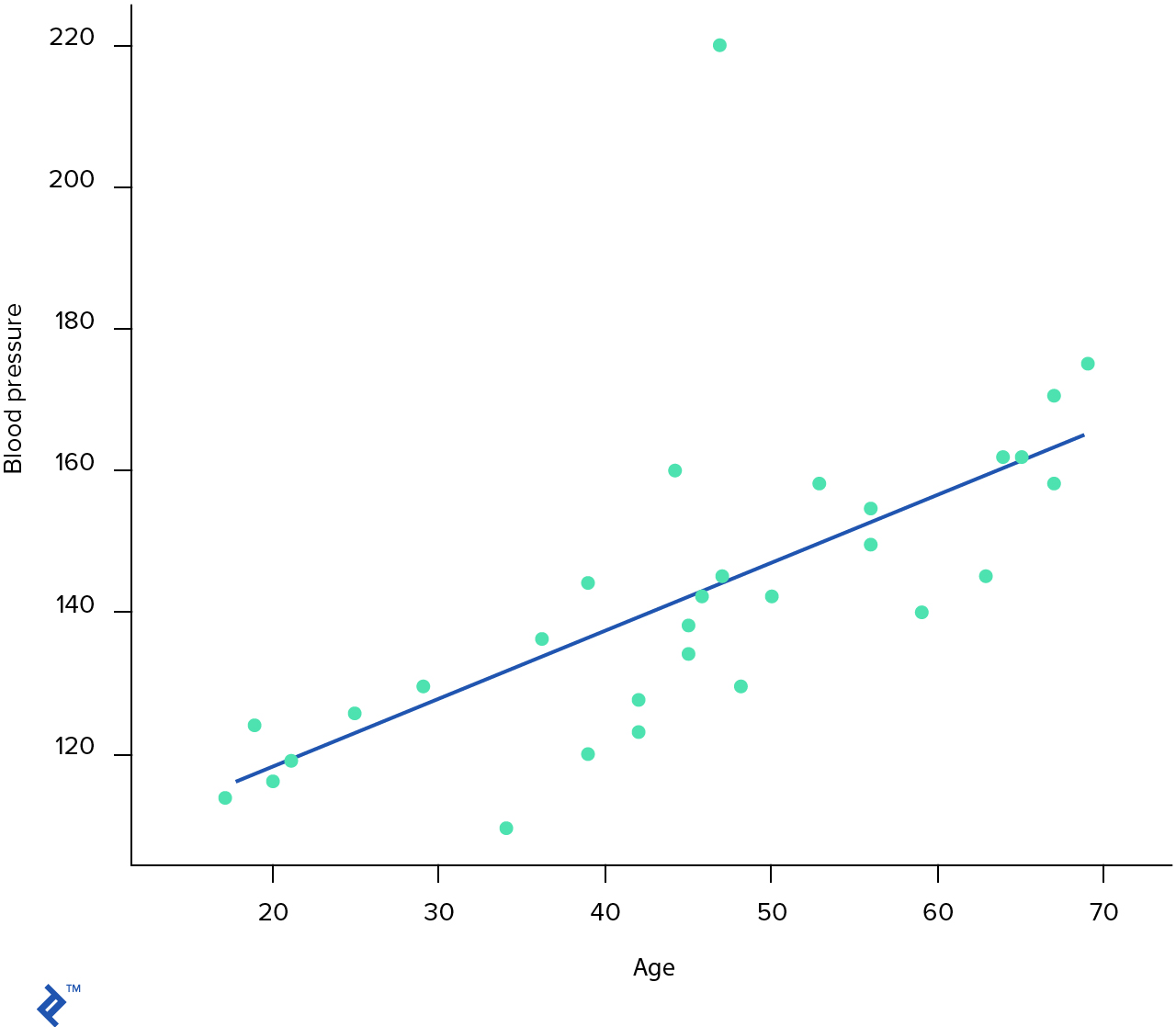
print( 'Predicted blood pressure at 25 y.o.   = ', regr.predict(25) )
print( 'Predicted blood pressure at 45 y.o.   = ', regr.predict(45) )
print( 'Predicted blood pressure at 27 y.o.   = ', regr.predict(27) )
print( 'Predicted blood pressure at 34.5 y.o. = ', regr.predict(34.5) )
print( 'Predicted blood pressure at 78 y.o.   = ', regr.predict(78) )

Predicted blood pressure at 25 y.o.   =  [[ 122.98647692]]
Predicted blood pressure at 45 y.o.   =  [[ 142.40388395]]
Predicted blood pressure at 27 y.o.   =  [[ 124.92821763]]
Predicted blood pressure at 34.5 y.o. =  [[ 132.20974526]]
Predicted blood pressure at 78 y.o.   =  [[ 174.44260555]]

Types of Statistical Data

When working with data for machine learning problems, it is important to recognize different types of data. We may have numerical (continuous or discrete), categorical, or ordinal data.

Numerical data has meaning as a measurement. For example, age, weight, number of bitcoins that a person owns, or how many articles the person can write per month. Numerical data can be further broken down into discrete and continuous types.

• Discrete data represent data that can be counted with whole numbers, e.g., number of rooms in an apartment or number of coin flips.
• Continuous data can’t necessarily be represented with whole numbers. For example, if you’re measuring the distance you can jump, it may be 2 meters, or 1.5 meters, or 1.652245 meters.

Categorical data represent values such as person’s gender, marital status, country, etc. This data can take numerical value, but those numbers have no mathematical meaning. You cannot add them together.

Ordinal data can be a mix of the other two types, in that categories may be numbered in a mathematically meaningful way. A common example is ratings: Often we are asked to rate things on a scale of one to ten, and only whole numbers are allowed. While we can use this numerically—e.g., to find an average rating for something—we often treat the data as if it were categorical when it comes to applying machine learning methods to it.

Logistic Regression

Linear regression is an awesome algorithm which helps us to predict numerical values, e.g., the price of the house with the specific size and number of rooms. However, sometimes, we may also want to predict categorical data, to get answers to questions like:

• Is this a dog or a cat?
• Is this tumor malignant or benign?
• Is this wine good or bad?
• Is this email spam or not?

Or even:

• Which number is in the picture?
• Which category does this email belong to?

All these questions are specific to the classification problem. And the simplest classification algorithm is called logistic regression, which is eventually the same as linear regression except that it has a different hypothesis.

First of all, we can reuse the same linear hypothesis $h_{\theta }\left(x\right)={\theta }^{T}X$ (this is in vectorized form). Whereas linear regression may output any number in the interval $[a,b]$, logistic regression can only output values in $[-1,1]$, which is the probability of the object falling in a given category or not.

Using a sigmoid function, we can convert any numerical value to represent a value on the interval $[-1,1]$.

$$f\left(x\right)=\frac{1}{1+e^x}$$

Now, instead of $x$, we need to pass an existing hypothesis and therefore we will get:

$$f\left(x\right)=\frac{1}{1+e^{{\theta }_0+{\theta }_1\ast x_1+...+{\theta }_n\ast x_n}}$$

After that, we can apply a simple threshold saying that if the hypothesis is greater than zero, this is a true value, otherwise false.

$$h_{\theta }\left(x\right)=\{\begin{array}{cc}1& \text{if}{\theta }^{T}X>0\\ 0& \text{else}\end{array}$$

This means that we can use the same cost function and the same gradient descent algorithm to learn a hypothesis for logistic regression.

In our next machine learning algorithm example, we will advise the pilots of the space shuttle whether or not they should use automatic or manual landing control. We have a very small dataset—15 samples—which consists of six features and the ground truth.

In machine learning algorithms, the term “ground truth” refers to the accuracy of the training set’s classification for supervised learning techniques.

Our dataset is complete, meaning that there are no missing features; however, some of the features have a “*” instead of the category, which means that this feature does not matter. We will replace all such asterisks with zeroes.

from sklearn.linear_model import LogisticRegression

# Data
data_path = os.path.join(os.getcwd(), "data/shuttle-landing-control.csv")
dataset = read_csv(data_path, header=None, 
                    names=['Auto', 'Stability', 'Error', 'Sign', 'Wind', 'Magnitude', 'Visibility'],
                    na_values='*').fillna(0)

# Prepare features
X = dataset[['Stability', 'Error', 'Sign', 'Wind', 'Magnitude', 'Visibility']]
y = dataset[['Auto']].values.reshape(1, -1)[0]

model = LogisticRegression()
model.fit(X, y)

# For now, we're missing one important concept. We don't know how well our model 
# works, and because of that, we cannot really improve the performance of our hypothesis. 
# There are a lot of useful metrics, but for now, we will validate how well 
# our algorithm performs on the dataset it learned from.
"Score of our model is %2.2f%%" % (model.score(X, y) * 100)

Score of our model is 73.33%

Validation?

In the previous example, we validated the performance of our model using the learning data. However, is this now a good option, given that our algorithm can either underfit of overfit the data? Let’s take a look at the simpler example when we have one feature which represents the size of a house and another which represents its price.

from sklearn.pipeline import make_pipeline
from sklearn.preprocessing import PolynomialFeatures
from sklearn.linear_model import LinearRegression
from sklearn.model_selection import cross_val_score

# Ground truth function
ground_truth = lambda X: np.cos(15 + np.pi * X)

# Generate random observations around the ground truth function
n_samples = 15
degrees = [1, 4, 30] 

X = np.linspace(-1, 1, n_samples)
y = ground_truth(X) + np.random.randn(n_samples) * 0.1

plt.figure(figsize=(14, 5))

models = {}

# Plot all machine learning algorithm models
for idx, degree in enumerate(degrees):
    ax = plt.subplot(1, len(degrees), idx + 1)
    plt.setp(ax, xticks=(), yticks=())
    
    # Define the model
    polynomial_features = PolynomialFeatures(degree=degree)
    model = make_pipeline(polynomial_features, LinearRegression())
    
    models[degree] = model
    
    # Train the model
    model.fit(X[:, np.newaxis], y)
    
    # Evaluate the model using cross-validation
    scores = cross_val_score(model, X[:, np.newaxis], y)
    
    X_test = X
    plt.plot(X_test, model.predict(X_test[:, np.newaxis]), label="Model")
    plt.scatter(X, y, edgecolor='b', s=20, label="Observations")
    
    plt.xlabel("x")
    plt.ylabel("y")
    plt.ylim((-2, 2))
    
    plt.title("Degree {}\nMSE = {:.2e}".format(
        degree, -scores.mean()))

plt.show()

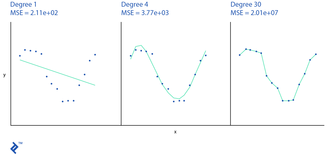
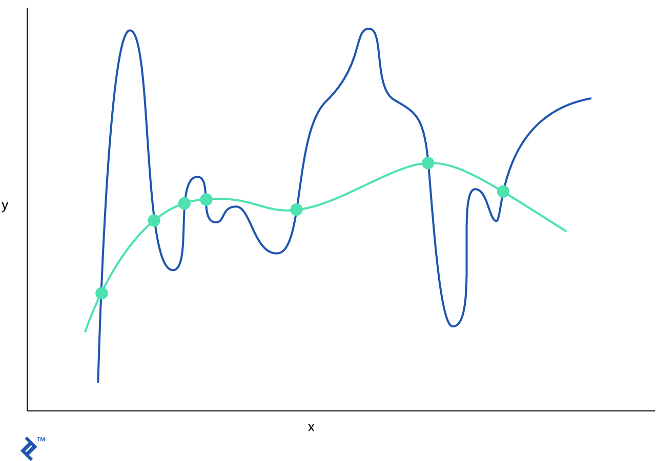
The machine learning algorithm model is underfitting if it can generalize neither the training data nor new observations. In the example above, we use a simple linear hypothesis which does not really represent the actual training dataset and will have very poor performance. Usually, underfitting is not discussed as it can be easily detected given a good metric.

If our algorithm remembers every single observation it was shown, then it will have poor performance on new observations outside of the training dataset. This is called overfitting. For example, a 30th-degree polynomial model passes through the most of the points and has a very good score on the training set, but anything outside of that would perform badly.

Our dataset consists of one feature and is simple to plot in 2D space; however, in real life, we may have datasets with hundreds of features, which makes them impossible to plot visually in Euclidean space. What other options do we have in order to see if the model is underfitting or overfitting?

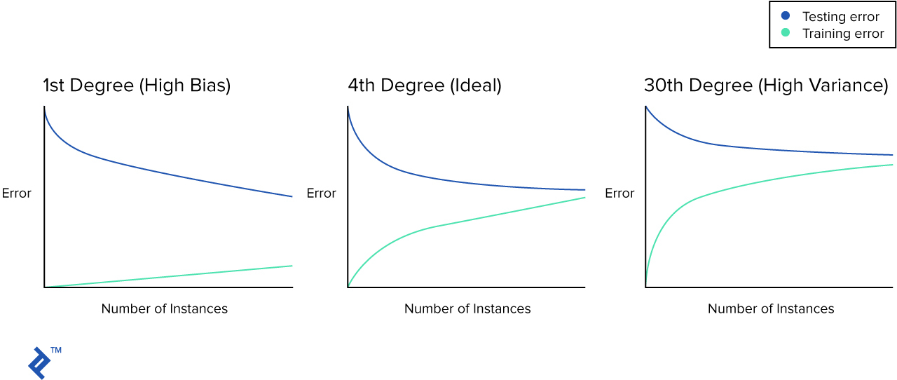
It’s time to introduce you to the concept of the learning curve. This is a simple graph that plots the mean squared error over the number of training samples.

In learning materials you will usually see graphs similar to these:

However, in real life, you may not get such a perfect picture. Let’s plot the learning curve for each of our models.

from sklearn.model_selection import learning_curve, ShuffleSplit

# Plot learning curves
plt.figure(figsize=(20, 5))

for idx, degree in enumerate(models):
    ax = plt.subplot(1, len(degrees), idx + 1)
    
    plt.title("Degree {}".format(degree))
    plt.grid()
    
    plt.xlabel("Training examples")
    plt.ylabel("Score")
    
    train_sizes = np.linspace(.6, 1.0, 6)
    
    # Cross-validation with 100 iterations to get a smoother mean test and training
    # score curves, each time with 20% of the data randomly selected as a validation set.
    cv = ShuffleSplit(n_splits=100, test_size=0.2, random_state=0)
    
    model = models[degree]
    train_sizes, train_scores, test_scores = learning_curve(
        model, X[:, np.newaxis], y, cv=cv, train_sizes=train_sizes, n_jobs=4)
    
    train_scores_mean = np.mean(train_scores, axis=1)
    test_scores_mean = np.mean(test_scores, axis=1)
    
    plt.plot(train_sizes, train_scores_mean, 'o-', color="r",
             label="Training score")
    plt.plot(train_sizes, test_scores_mean, 'o-', color="g",
             label="Test score")
    
    plt.legend(loc = "best")

plt.show()

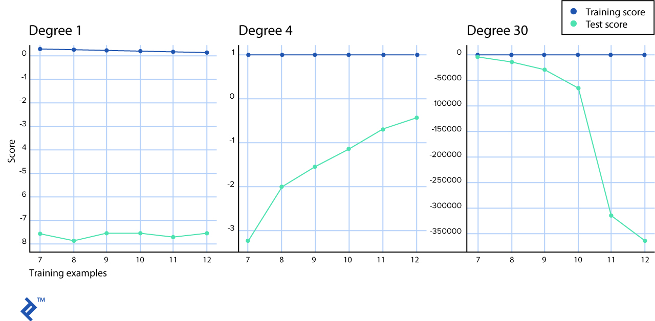
In our simulated scenario, the blue line, which represents the training score, seems like a straight line. In reality, it still slightly decreases—you can actually see this in the first-degree polynomial graph, but in the others it’s too subtle to tell at this resolution. We at least clearly see that there is a huge gap between learning curves for training and test observations with a “high bias” scenario.

On the “normal” learning rate graph in the middle, you can see how training score and test score lines come together.

And on the “high variance” graph, you can see that with a low number of samples, the test and training scores are very similar; however, when you increase the number of samples, the training score remains almost perfect while the test score grows away from it.

---

We can fix underfitting models (also called models with high bias) if we use a non-linear hypothesis, e.g., the hypothesis with more polynomial features.

Our overfitting model (high variance) passes through every single example it is shown; however, when we introduce test data, the gap between learning curves widens. We can use regularization, cross-validation, and more data samples to fix overfitting models.

Cross-validation

One of the common practices to avoid overfitting is to hold onto part of the available data and use it as a test set. However, when evaluating different model settings, such as the number of polynomial features, we are still at risk of overfitting the test set because parameters can be tweaked to achieve the optimal estimator performance and, because of that, our knowledge about the test set can leak into the model. To solve this problem, we need to hold onto one more part of the dataset, which is called the “validation set.” Training proceeds on the training set and, when we think that we’ve achieved the optimal model performance, we can make a final evaluation utilizing the validation set.

However, by partitioning the available data into three sets, we dramatically reduce the number of samples that can be used for training the models, and the results can depend on a particular random choice for the training-validation pair of sets.

One solution to this problem is a procedure called cross-validation. In standard $k$-fold cross-validation, we partition the data into $k$ subsets, called folds. Then, we iteratively train the algorithm on $k-1$ folds while using the remaining fold as the test set (called the “holdout fold”).

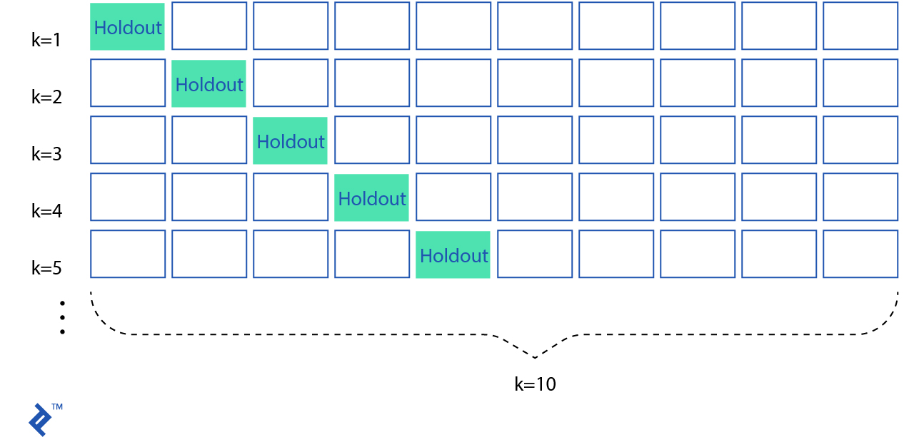
Cross-validation allows you to tune parameters with only your original training set. This allows you to keep your test set as a truly unseen dataset for selecting your final model.

There are a lot more cross-validation techniques, like leave P out, stratified $k$-fold, shuffle and split, etc. but they’re beyond the scope of this article.

Regularization

This is another technique that can help solve the issue of model overfitting. Most of the datasets have a pattern and some noise. The goal of the regularization is to reduce the influence of the noise on the model.

There are three main regularization techniques: Lasso, Tikhonov, and elastic net.

L1 regularization (or Lasso regularization) will select some features to shrink to zero, such that they will not play any role in the final model. L1 can be seen as a method to select important features.

L2 regularization (or Tikhonov regularization) will force all features to be relatively small, such that they will provide less influence on the model.

Elastic net is the combination of L1 and L2.

Normalization (Feature Scaling)

Feature scaling is also an important step while preprocessing the data. Our dataset may have features with values $[-\infty ,\infty ]$ and other features with a different scale. This is a method to standardize the ranges of independent values.

Feature scaling is also an important process to improve the performance of the learning models. First of all, gradient descent will converge much faster if all of the features are scaled to the same norm. Also, a lot of algorithms—for example, support vector machines (SVM)—work by calculating the distance between two points and if one of the features has broad values, then the distance will be highly influenced by this feature.

Support Vector Machines

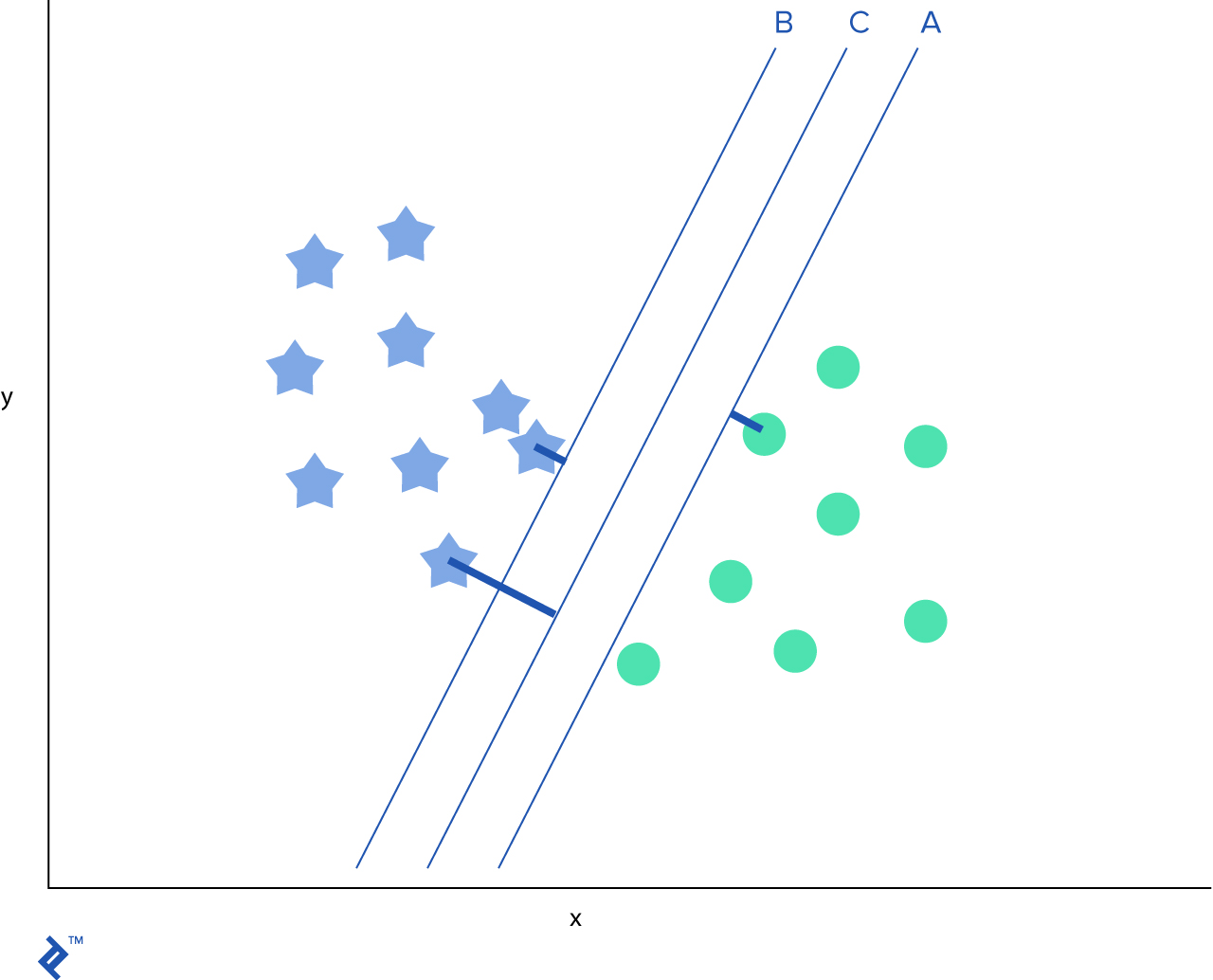
SVM is yet another broadly popular machine learning algorithm which can be used for classification and regression problems. In SVM, we plot each observation as a point in $n$-dimensional space where $n$ is the number of features we have. The value of each feature is the value of particular coordinates. Then, we try to find a hyperplane that separates two classes well enough.

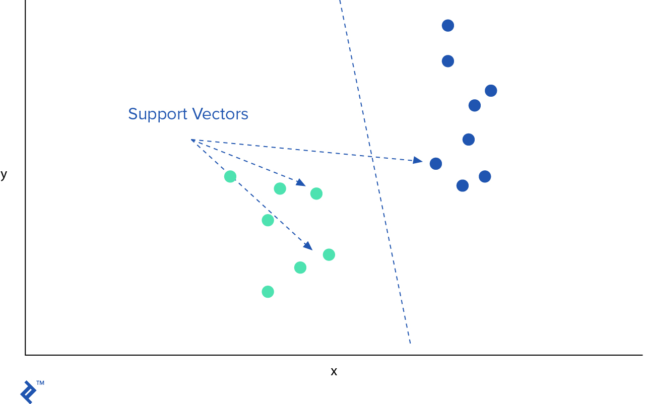
After we identify the best hyperplane, we want to add margins, which would separate the two classes further.

SVM is very effective where the number of features is very high or if the number of features is larger then the number of data samples. However, since SVM operates on a vector basis, it is crucial to normalize the data prior the usage.

Neural Networks

Neural network algorithms are probably the most exciting field of machine learning studies. Neural networks try to mimic how the brain’s neurons are connected together.

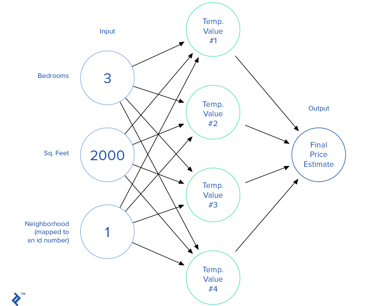
This is how a neural network looks. We combine a lot of nodes together where each node takes a set of inputs, apply some calculations on them, and output a value.

There are a huge variety of neural network algorithms for both supervised and unsupervised learning. Neural networks can be used to drive autonomous cars, play games, land airplanes, classify images, and more.

The Infamous Titanic

The RMS Titanic was a British passenger liner that sank in the North Atlantic Ocean on April 15th, 1912 after it collided with an iceberg. There were about 2,224 crew and passengers, and more than 1,500 died, making it one of the deadliest commercial maritime disasters of all time.

Now, since we understand the intuition behind the most basic machine learning algorithms used for classification problems, we can apply our knowledge to predict the survival outcome for those on board the Titanic.

Our dataset will be borrowed from the Kaggle data science competitions platform.

import os
from pandas import read_csv, concat

# Load data
data_path = os.path.join(os.getcwd(), "data/titanic.csv")
dataset = read_csv(data_path, skipinitialspace=True)

dataset.head(5)

	PassengerId	Survived	Pclass	Name	Sex	Age	SibSp	Parch	Ticket	Fare	Cabin	Embarked
0	1	0	3	Braund, Mr. Owen Harris	male	22.0	1	0	A/5 21171	7.2500	NaN	S
1	2	1	1	Cumings, Mrs. John Bradley (Florence Briggs Th...	female	38.0	1	0	PC 17599	71.2833	C85	C
2	3	1	3	Heikkinen, Miss. Laina	female	26.0	0	0	STON/O2. 3101282	7.9250	NaN	S
3	4	1	1	Futrelle, Mrs. Jacques Heath (Lily May Peel)	female	35.0	1	0	113803	53.1000	C123	S
4	5	0	3	Allen, Mr. William Henry	male	35.0	0	0	373450	8.0500	NaN	S

Our first step would be to load and explore the data. We have 891 test records; each record has the following structure:

• passengerId – ID of the passenger on board
• survival – Whether or not the person survived the crash
• pclass – Ticket class, e.g., 1st, 2nd, 3rd
• gender – Gender of the passenger: Male or female
• name – Title included
• age – Age in years
• sibsp – Number of siblings/spouses aboard the Titanic
• parch – Number of parents/children aboard the Titanic
• ticket – Ticket number
• fare – Passenger fare
• cabin – Cabin number
• embarked – Port of embarkation

This dataset contains both numerical and categorical data. Usually, it is a good idea to dive deeper into the data and, based on that, come up with assumptions. However, in this case, we will skip this step and go straight to predictions.

import pandas as pd

# We need to drop some insignificant features and map the others.
# Ticket number and fare should not contribute much to the performance of our models.
# Name feature has titles (e.g., Mr., Miss, Doctor) included.
# Gender is definitely important.
# Port of embarkation may contribute some value.
# Using port of embarkation may sound counter-intuitive; however, there may 
# be a higher survival rate for passengers who boarded in the same port.

dataset['Title'] = dataset.Name.str.extract(' ([A-Za-z]+)\.', expand=False)
dataset = dataset.drop(['PassengerId', 'Ticket', 'Cabin', 'Name'], axis=1)

pd.crosstab(dataset['Title'], dataset['Sex'])

Title \ Sex	female	male
Capt	0	1
Col	0	2
Countess	1	0
Don	0	1
Dr	1	6
Jonkheer	0	1
Lady	1	0
Major	0	2
Master	0	40
Miss	182	0
Mlle	2	0
Mme	1	0
Mr	0	517
Mrs	125	0
Ms	1	0
Rev	0	6
Sir	0	1

# We will replace many titles with a more common name, English equivalent,
# or reclassification
dataset['Title'] = dataset['Title'].replace(['Lady', 'Countess','Capt', 'Col',\
  'Don', 'Dr', 'Major', 'Rev', 'Sir', 'Jonkheer', 'Dona'], 'Other')

dataset['Title'] = dataset['Title'].replace('Mlle', 'Miss')
dataset['Title'] = dataset['Title'].replace('Ms', 'Miss')
dataset['Title'] = dataset['Title'].replace('Mme', 'Mrs')
    
dataset[['Title', 'Survived']].groupby(['Title'], as_index=False).mean()

	Title	Survived
0	Master	0.575000
1	Miss	0.702703
2	Mr	0.156673
3	Mrs	0.793651
4	Other	0.347826

# Now we will map alphanumerical categories to numbers
title_mapping = { 'Mr': 1, 'Miss': 2, 'Mrs': 3, 'Master': 4, 'Other': 5 }
gender_mapping = { 'female': 1, 'male': 0 }
port_mapping = { 'S': 0, 'C': 1, 'Q': 2 }

# Map title
dataset['Title'] = dataset['Title'].map(title_mapping).astype(int)

# Map gender
dataset['Sex'] = dataset['Sex'].map(gender_mapping).astype(int)

# Map port
freq_port = dataset.Embarked.dropna().mode()[0]
dataset['Embarked'] = dataset['Embarked'].fillna(freq_port)
dataset['Embarked'] = dataset['Embarked'].map(port_mapping).astype(int)

# Fix missing age values
dataset['Age'] = dataset['Age'].fillna(dataset['Age'].dropna().median())

dataset.head()

	Survived	Pclass	Sex	Age	SibSp	Parch	Fare	Embarked	Title
0	0	3	0	22.0	1	0	7.2500	0	1
1	1	1	1	38.0	1	0	71.2833	1	3
2	1	3	1	26.0	0	0	7.9250	0	2
3	1	1	1	35.0	1	0	53.1000	0	3
4	0	3	0	35.0	0	0	8.0500	0	1

At this point, we will rank different types of machine learning algorithms in Python by using scikit-learn to create a set of different models. It will then be easy to see which one performs the best.

• Logistic regression with varying numbers of polynomials
• Support vector machine with a linear kernel
• Support vector machine with a polynomial kernel
• Neural network

For every single model, we will use $k$-fold validation.

from sklearn.model_selection import KFold, train_test_split
from sklearn.pipeline import make_pipeline
from sklearn.preprocessing import PolynomialFeatures, StandardScaler

from sklearn.neural_network import MLPClassifier
from sklearn.svm import SVC

# Prepare the data
X = dataset.drop(['Survived'], axis = 1).values
y = dataset[['Survived']].values

X = StandardScaler().fit_transform(X)

X_train, X_test, y_train, y_test = train_test_split(X, y, test_size=0.2, random_state = None)

# Prepare cross-validation (cv)
cv = KFold(n_splits = 5, random_state = None)

# Performance
p_score = lambda model, score: print('Performance of the %s model is %0.2f%%' % (model, score * 100))

# Classifiers
names = [
    "Logistic Regression", "Logistic Regression with Polynomial Hypotheses",
    "Linear SVM", "RBF SVM", "Neural Net",
]

classifiers = [
    LogisticRegression(),
    make_pipeline(PolynomialFeatures(3), LogisticRegression()),
    SVC(kernel="linear", C=0.025),
    SVC(gamma=2, C=1),
    MLPClassifier(alpha=1),
]

# iterate over classifiers
models = []
trained_classifiers = []
for name, clf in zip(names, classifiers):
    scores = []
    for train_indices, test_indices in cv.split(X):
        clf.fit(X[train_indices], y[train_indices].ravel())
        scores.append( clf.score(X_test, y_test.ravel()) )
    
    min_score = min(scores)
    max_score = max(scores)
    avg_score = sum(scores) / len(scores)
    
    trained_classifiers.append(clf)
    models.append((name, min_score, max_score, avg_score))
    
fin_models = pd.DataFrame(models, columns = ['Name', 'Min Score', 'Max Score', 'Mean Score'])

fin_models.sort_values(['Mean Score']).head()

	Name	Min Score	Max Score	Mean Score
2	Linear SVM	0.793296	0.821229	0.803352
0	Logistic Regression	0.826816	0.860335	0.846927
4	Neural Net	0.826816	0.860335	0.849162
1	Logistic Regression with Polynomial Hypotheses	0.854749	0.882682	0.869274
3	RBF SVM	0.843575	0.888268	0.869274

Ok, so our experimental research says that the SVM classifier with a radial basis function (RBF) kernel performs the best. Now, we can serialize our model and re-use it in production applications.

import pickle

svm_model = trained_classifiers[3]

data_path = os.path.join(os.getcwd(), "best-titanic-model.pkl")
pickle.dump(svm_model, open(data_path, 'wb'))

Machine learning is not complicated, but it’s a very broad field of study, and it requires knowledge of math and statistics in order to grasp all of its concepts.

Right now, machine learning and deep learning are among the hottest topics of discussion in Silicon Valley, mainly because they can automate many repetitive tasks including speech recognition, driving vehicles, financial trading, caring for patients, cooking, marketing, and so on.

Now you can take this knowledge and solve challenges on Kaggle.

This was a very brief introduction to supervised machine learning algorithms. Luckily, there are a lot of online courses and information about machine learning algorithms. I personally would recommend starting with Andrew Ng’s course on Coursera.

BY VLADYSLAV MILLIER - FREELANCE SOFTWARE ENGINEER

Source: https://www.toptal.com/machine-learning/supervised-machine-learning-algorithms